Evaluation of Classical Statistical Methods for Analyzing BS-Seq Data

Hengrui Luo, Shili Lin

1. Department of Statistics, The Ohio State University, Columbus, OH, USA

*   Correspondence: Shili Lin

Received: May 23, 2018 | Accepted: November 26, 2018 | Published: December 10, 2018

OBM Genetics 2018, Volume 2, Issue 4 doi: 10.21926/obm.genet.1804053

Academic Editors: Stéphane Viville and Marcel Mannens

Special Issue: Epigenetic Mechanisms in Health and Disease

Recommended citation: Luo H, Lin S. Evaluation of Classical Statistical Methods for Analyzing BS-Seq Data. OBM Genetics 2018;2(4):053; doi:10.21926/obm.genet.1804053.

© 2018 by the authors. This is an open access article distributed under the conditions of the Creative Commons by Attribution License, which permits unrestricted use, distribution, and reproduction in any medium or format, provided the original work is correctly cited.

1. Introduction

DNA methylation is key to the normal development of cells [1,2,3] and may control phenotypes that are heritable across generations [4]. Biological studies have [Lister et.al] indicated the existence of a close relationship between CpG (5'C-phosphate-G3') methylation and regulation of gene expression [5,6]. However, aberrant DNA methylation patterns, especially those that are acquired later in life and in gene promoters, may be adversely linked to human health and disease; therefore, DNA methylation has become a central research topic in the field of epigenetics over the past decade [7,8]. In particular, it has been shown that promoter hypermethylation can lead to deregulation of the transcription of cancer suppressor genes [7,8]. Studies have also shown that increased methylation of CpG islands is correlated with the functioning of molecular pathways that play a central role in common diseases, such as colorectal cancer [9]. More recent epigenetic studies have also shown that disease-associated variants can influence DNA methylation levels in transcription regions [10]. An abundance of biological evidence points firmly to the role of DNA methylation in the development of human diseases, and its potential as biomarkers of such conditions.

The recent development of various bisulfite sequencing (BS-seq) technologies has led to the production of single-base resolution data for measuring DNA methylation [1]. These techniques involve the conversion of unmethylated cytosines to detect methylation at each base pair; the result is typically represented as a pair of counts comprising the total reads and methylated reads at each site [11]. A number of algorithms have been proposed to handle various aspects of preprocessing that allow organization of the data into a typical contingency table (Table 1). In particular, several approaches have been proposed for alignment, an important step in data preprocessing. This is especially challenging for standard alignment tools due to bias created by reads with unmethylated cytosines. Algorithms proposed to deal with this specific issue include BSMAP [12], GSNAP [13], Bismark [14], and BRAT [15]. In recent years, visualization tools have also been developed to aid the understanding of genome-wide methylation data and interpretation of analysis results; these include MethGo [16] and ViewBS [17]. Various new statistical methods that have been developed specifically for analyzing BS-seq data have been comprehensively reviewed [18] and a comparative study of some of these methods has also been reported [19]. Despite these efforts, a number of statistical challenges remain when analyzing and drawing inferences from DNA methylation data [20].

Methylation counts at a single site (which may include CHG and CHH in addition to CpG, where H represents A, T, or C) can be modeled as a random variable from a binomial distribution with the methylation probability (Ρ) and the number of total reads (n) as the success probability and the number of trials, respectively. The probability of this binomial distribution reflects the methylation level at the site. The ratio of methylated and total reads at a specific site can be used as a (maximum-likelihood) estimate of the methylation probability [20]. Under the binomial model, hypothesis-testing can be conducted at each site, leading to the potential detection of differentially methylated cytosines (DMCs). This problem can be framed statistically by testing whether the methylation probabilities from two binomial populations differ significantly. Despite the fact that detecting an entire differentially methylated region (DMR) is frequently of greater interest [21], testing for DMCs is usually carried out instead (or at least as the first step). We note that site-by-site detection methods, which form the subject of this study, do not take spatial dependency into consideration.

It is known that epigenomes are known to vary among individuals, even within the same population[4]. These differences give rise to the potential issue of biological variation even among samples within a group (i.e. all samples under a specific condition, such as all healthy individuals or all having a particular disease). Regions on chromosomes that are inherently more variable across different samples will lead to higher false positive rates when statistical tests that ignore such variability are applied [22,23,24]. When there are only a few biological replicates, the potential loss of power is also a concern with single-site analysis methods because spatial correlations are ignored [22,23,25,26].

Despite the problems discussed here, site-wise analysis and methods that do not take biological variation (even when there are replicates) into consideration continue to be used for DNA methylation analysis. This is because such analysis can be carried out by simple, traditional, and well-known methods that biological scientists can “confidently” rely on, such as Fisher’s exact (FE) test. On the other hand, in the rush to develop new statistical methodology that takes between-sample variability into account, the suitability of the FE test for analyzing BS-seq data has not been investigated by computational and data scientists.

To fill this void, we have evaluated the FE test, along with several other single-site testing methods, to ascertain their appropriateness and compare their performance, with or without availability of replicates. The FE test has recently been recommended without critique as the de facto method for analyzing non-replicated BS-seq data [27]; this highlights the importance of our current study, which will provide biological scientists with a much-needed guide for selecting the appropriate method for analyzing their DNA methylation data when biological replicates are not available. Even when biological replicates are available but a simple test is required, this study will further our understanding of the operational characteristics of these traditional hypothesis-testing methods, especially regarding the existence of inflated type I error and/or reduced power.

1.1. Fixed Margins Assumption in Fisher’s Exact Test

The FE test is one of the most frequently used methods for single-site analysis to detect DMCs. This method relies on the assumption of fixed margins of a contingency table (Table 1); hence, it is usually referred to as a conditional test. It has been argued that a conditional test is better applied under an appropriate sampling scheme [28,29]; however, if the sampling scheme is violated, then tests without the erroneous conditions would perform better in terms of power while preserving nominal type I errors [30,31,32].

Data generated from BS-seq studies are not conditioned on fixed margins, as one does not know, beforehand, the sum of methylated reads in the two conditions. Therefore, the assumption of fixed margins in the contingency table is violated and it is therefore doubtful that the margins of the contingency table are ancillary statistics (i.e. do not contain information about methylation intensities) as required by the FE test and other conditional tests [32,33]. To carefully evaluate this issue, in this study we evaluated the properties of the FE test, together with several other tests, for their appropriateness for analyzing BS-seq data.

Table 1 A typical 2 x 2 contingency table.

For Fisher’s exact test, the row sums (margins r₁ + r₂ and f₁ + f₂) as well as the column sums (margins n₁=f₁ + r₁ and n₂=f₂ + r₂) are assumed to be fixed; the test is carried out conditioned on these margins.

2. Methods of Comparison

In this study, we evaluated three testing methods. The first, the FE test, was chosen because of its convenience and popularity, despite its conditional nature as discussed earlier [1]. The second is also a frequently used traditional test, the chi-squared (CS) test. This test is typically used in a large-sample situation, but there is also a small-sample Monte Carlo version although it can be computationally expensive and can be sensitive to the choice of running parameters [34]. We chose to include the CS test in this investigation because it can be viewed as a computationally efficient large-sample approximation of the conditional FE test; thus, we included it as a “reference” without invoking the computationally expensive Monte Carlo version. The third, and final method, the Storer–Kim (SK) test, is an approximate unconditional test for comparing two binomial probabilities [35]. This approximate version of an exact unconditional test [36] was proposed to alleviate the concern regarding the computational cost of the exact test. In addition to the three tests that we compared for the detection of DMCs, we also used Welch’s t-test to address the issue of biological variation, although we note that this test has its own drawback in that it does not take the total reads into account, a disadvantage that has been criticized by others [18]. Here, we describe each of these methods briefly. To be specific, we tested the hypothesis:

H₀:p₁ versus H_a:p₁ ≠ p₂,

where p₁ and p₂ denote the methylation levels (i.e. binomial probabilities) under two conditions (or two populations).

2.1. Fisher’s Exact Test

The FE test [37] is a classical test for the difference between two binomial probabilities based on data that can be organized into a contingency table like the one used to analyze DNA methylation data (Table 1). When some counts in the contingency table are small, the FE test is a popular choice instead of its large-sample counterpart, the CS test. Using the notation in Table 1, its P-value for testing H₀ versus H_a is calculated according to the following formula:

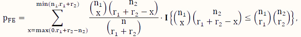
where x is an indexing variable, and I is the usual indicator function taking the value of 1 (or 0) depending on whether the condition in the curly brackets is satisfied (or not). Note that this test assumes that both the row sums and the column sums (Table 1) are fixed, which is essentially a test based on the hypergeometric sampling scheme.

2.2. Chi-Squared Test

The CS test [38] is a large-sample approximation of the FE test. Again, using the notation in Table 1, the test statistic is calculated according to the following formula:

which is assumed to follow a distribution under the null hypothesis . The P-value can then be determined by computing the tail probability of the distribution.

2.3. Storer-Kim Test

In contrast to conditional tests, such as the FE test, here, we consider unconditional tests, which have been shown to have better control of type I error as well as higher power if the sample scheme does not warrant the appropriateness of the assumption of a conditional test [31,32,33,39]. To address the issue of computational intensity of an exact unconditional test [36], we consider the SK test [35], which is an approximate unconditional test. Its P-value is calculated according to the following formula:

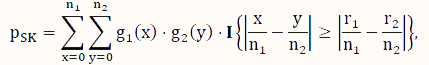
where x and y are indexing variables, I is the indicator function as defined earlier, and g₁ and g₂ are the probability functions of the binomial distributions Binom($n_1,\hat p$) and Binom($n_2,\hat p$), respectively, where .

2.4. Welch’s t-Test

Welch’s t (WT)-test is a two-sample mean test without assuming the variances of the two populations being equal. Its test statistic is calculated according to the following formula:

,

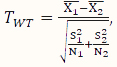where and , respectively, are the sizes of the samples from the two populations (conditions) under investigation, and  and are the mean and variance of the sample from the first population. Note that the representation in Table 1 only depicts data for a single sample, whereas in the current setting, we have biological replicates and thus, our data should be represented by N₁ tables, where x_i = r_i/n_i, i=1, 2, ..., N₁, using the notation shown in Table 1. We define and similarly. The P-value of the test statistic is obtained from a t-distribution with an appropriately calculated degree of freedom [40]. This test was adopted as a reference test in our second simulation study where there is between-sample variability, as it takes such variability into account rather than pooling data from samples within a group and is known to be robust.

3. Simulation and Theoretical Studies

Extensive studies were carried out to comprehensively compare and contrast the methods. Specifically, two empirical studies and one theoretical study were conducted. The first study was carried out using simulated data based on the characteristics of a whole genome bisulfite sequencing (WGBS) dataset [1]. This study was designed to evaluate the performance of the FE, CS, and SK tests for detecting DMCs. The second study utilized data simulated from a model that assumes spatial correlation and between-sample variability [41]. The goal of this investigation was to gauge the performance of the methods in non-ideal, but more realistic situations with patient samples. The last study was theoretical, in which the rejection regions from the three methods were calculated and compared for a variety of methylation probabilities and total number of reads.

3.1. Study 1: Detection of DMCs under Idealized Conditions

This simulation study was based on the results from our analysis of a WGBS dataset [1] in which the methylation levels of two cell lines (H1 and IMR90) were compared; details of the analyses and results of this dataset are given in Section 4. In this simulation, we treated the sites that were detected as DMCs by all methods as “true DMCs” and the rest as “null sites”. Note that this method is not recommended for the designation of DMCs in any real data analysis; rather, this choice was made to facilitate a fair and objective comparison in our in-silico study using sites that can be detected using all three methods. As such, our simulation scheme may be regarded as generating an independent dataset for “validation” of the overlapping sites. We randomly selected 10% of the “true DMCs” and 10% of the “null sites” for inclusion in the simulation. In the case of a true DMC, we used the estimated (proportion of methylated reads in the H1 cell line) and (proportion of methylated reads in the IMR90 cell line) as the true binomial probabilities. Together with their respective total reads n₁ and n₂, we simulated realizations (the r values shown in Table 1) from the two binomial distributions; these were the methylated reads. Note that the total reads reflect the sequencing depth of the experiment and were taken directly from the real data study; these values varied from site to site (the histograms of the read counts for all sites from the H1 and IMR90 cell lines are shown in Supplementary Figure S8). For a “null site’, and were both set as the pooled estimate so that . The rest of the procedure for the simulation was the same as that used for a “true DMC” site.

We applied the FE, CS and SK tests to each simulated binomial dataset. Since the “ground truths” were known, we were able to compute the power and type I error based on the testing results for each method. We defined power as the proportion of rejections among all true DMCs and the type I error rate as the proportion of rejections among all null sites. The results, presented in Figure 1, show that the type I error rates for all three tests were well below the nominal level of 0.05: all three tests were conservative, with the CS test being the most extreme. In terms of power, the SK test achieved the highest, followed by the FE test, which outperforms the CS test. Although the differences in the power were small, the number of additional DMCs detected were nonetheless substantial given the large number of sites considered (in the order of millions).

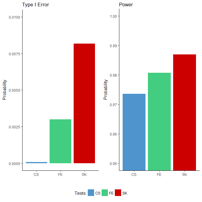
Figure 1 Comparison of type I error rates (left side) and power (right side) among the Storer–Kim (SK), Fisher’s exact (FE) and chi-squared (CS) tests using data simulated based on the characteristics of a whole genome bisulfite sequencing study [1]. Note that these two figures are not drawn to the same scale.

3.2. Study 2: Detection of DMCs in the Presence of Spatial Correlation and Between-Sample Variability

As discussed earlier, the first set of simulations were carried out under idealized conditions, in which methylated reads follow independent binomial distributions across sites and there was no between-sample variability (i.e. as if only one sample was available under each condition). In this second study, we simulated data from a more realistic model, in which spatial correlation and between-sample variation were assumed. Specifically, our simulation was modeled using a WGBS colon cancer dataset of six samples (3 cancer and 3 normal) that are available in the bsseqData Bioconductor package. For convenience, since the colon dataset is already linked to BSmooth [42], we used it to detect DMRs on chromosome 21 and treated all sites therein as DMCs and those outside of the DMRs as null sites. Together with the total read counts from the real data, we simulated 100 datasets under each of four variability scenarios following the data simulation procedure described in BCurve [41].

The results for type I error are presented in Figure 2, from which we found that the three tests investigated above all had inflated type I error, especially as the between-sample variability increased from scenario 1 (S1) to scenario 4 (S4). These results were as expected, because these tests do not allow for between-sample variability, the presence of which may be treated as “signals”. On the other hand, Welch’s t-test, being able to account for between-sample variability, was the closest to the nominal level of 0.05, regardless of the level of variability.

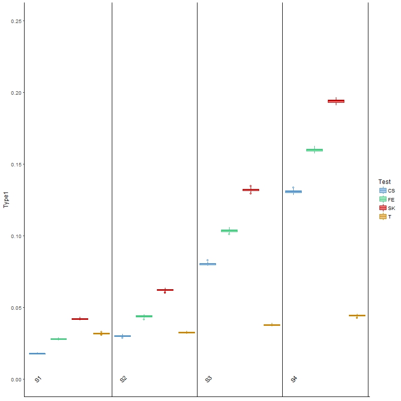
Figure 2 Boxplots of type I error rates for each of the four comparison methods over 100 simulated datasets modeled on a colon cancer dataset. The four scenarios considered, S1, S2, S3, S4, are arranged in increasing order of between-sample variability.

In terms of power, the results (Figure 3) of Welch’s t-test were as expected: as variability increased, the power for detecting DMCs decreased. It was, however, noted that the power was low, which was partially attributed to the ignorance of information contained in the spatial correlation. This general behavior was also observed for the other three tests, although the decrease in power was less drastic than that of the t-test. The SK test remained the most powerful, although its type I error was also the highest of all four scenarios among the three main comparison methods. Finally, the powers of these three methods were all higher than those of the t-test, but once again it was noted that all three had much larger type I error than the latter test. In summary, this investigation and the results show that the t-test is more appropriate for analyzing BS-seq data when there is a considerable amount of between-sample variability; however, it has low power, and is not applicable in a more general setting where covariate information is available, as we elaborate in the Discussion section.

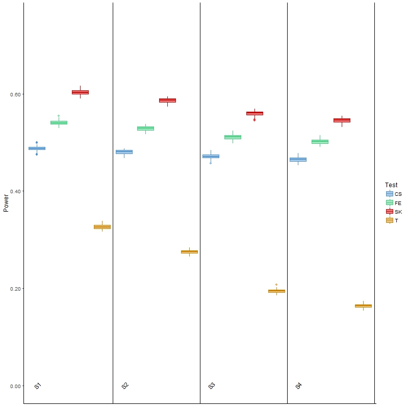
Figure 3 Boxplots of power for each of the four comparison methods over 100 simulated datasets modeled on a colon cancer dataset. The four scenarios considered, S1, S2, S3, S4, are arranged in increasing order of between-sample variability.

3.3. Study 3: Theoretical Investigation of the Methods for Detecting DMCs

In the first two studies, we carried out simulations to evaluate and compare the FE, CS and SK tests for detecting DMCs. The results all showed that the SK test had the highest power while still being able to control the type I error. However, whether the superiority of the SK test is due to a particular simulation or whether it is more inherent in testing for DMCs remained open to debate. To answer this question, we carried out a theoretical analysis in our third study.

We considered two settings. In the first, the methylation probabilities, P₁ and P₂, were assumed to be fixed, and we were interested in investigating the power when we varied the total reads n₁ and n₂, reflecting the sequencing depth. The number of methylated reads, r₁ and r₂, were then inferred from each pair of (n₁, n₂). In the second setting, we fixed the total number of reads, n₁ and n₂, but varied the methylation probabilities, p₁ and p₂. In this case, the number of methylated reads, r₁ and r₂ were also derived for each pair of (p₁, p₂). Our aim was to understand how the interplay between sequencing depth and differential healthy control/disease individual methylation profiles influences the detection of DMCs.

For each of these settings described previously, we constructed the rejection region for each of the three tests. Note that a larger rejection region is indicative of a more powerful method when the nominal type I error rates are kept the same. In the first setting, in which the methylation probabilities p₁ and p₂ were fixed at 0.2 and 0.4, respectively, the results (Figure 4) showed that the SK test has the largest rejection region. Furthermore, the SK test was found to provide a more accurate method of identifying DMCs using data with a relatively small number of total reads (n₁, n₂) compared with the other two methods. The CS test was shown to provide the poorest performance. This observation held true for several other settings of p₁ and p₂ values (Supplementary Figures S1-S3). In the second setting, in which the total reads, n₁ and n₂, were both fixed at 25, the results (Figure 5) showed that the rejection region of the SK test was once again the largest, while the CS test remains the poorest performing method, most likely due to its inadequacy in small-sample scenarios. These results were also applicable to several other settings of the n₁ and n₂ values (Supplementary Figures S4-S6).

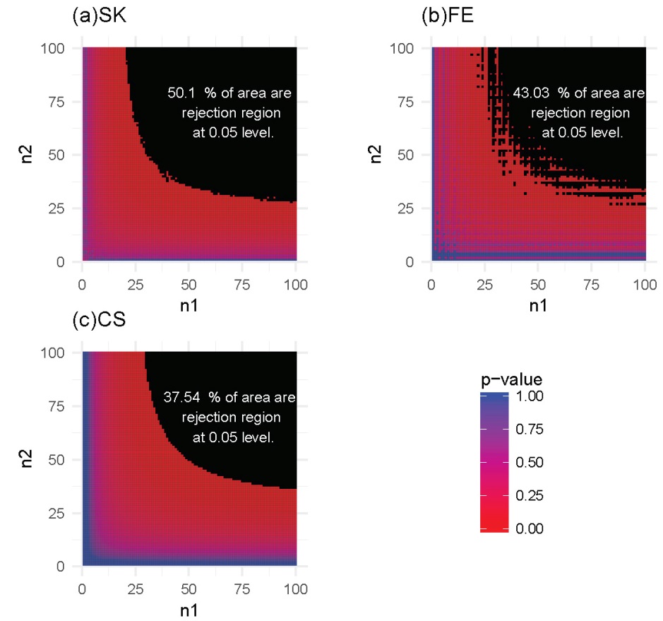
Figure 4 Heatmaps of P-values and rejection regions (those with P-values ≤0.05; shaded in black): (a) Storer–Kim (SK); (b) Fisher’s exact (FE); and (c) and chi-squared (CS) tests. The results are for a pair of p’s fixed at p₁=0.4 and p₂=0.2. For each method, the rejection region is the combination of (n₁, n₂) (in the range of 1-100) for which the DMC is declared. Note that the jagged line in (b) is due to the discrete nature of the FE test.

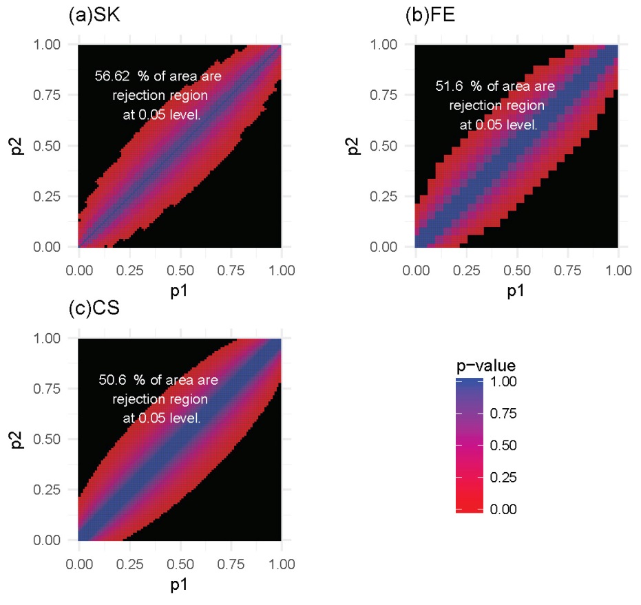
Figure 5 Heatmaps of P-values and rejection regions (those with P-values ≤0.05; shaded in black): (a) Storer–Kim (SK); (b) Fisher’s exact (FE); and (c) and chi-squared (CS) tests. The results are for a scenario in which the total number of reads is 25 in both samples. For each method, the rejection region is the combination of (p₁, p₂) (in the range of 0-1) for which the DMC is declared. Note that the jagged line in (b) is due to the discrete nature of the FE test.

In summary, our analysis shows that the SK test has the greatest ability to detect DMCs for data with low sequencing depth. Stated differently, compared to the other two methods, the SK test will have a greater power of detecting DMCs, for a study with a fixed sequencing depth, even with small differences in the methylation levels. In general, for a fixed sequencing depth, the larger the difference between the methylation levels, the greater the ability of all methods for detecting the difference, as expected. Similarly, for a fixed difference, the deeper the sequencing depth, the greater the power with which the difference will be detected, again for all methods.

4. Analysis of a Real Dataset

To corroborate our findings from the in-silico studies showing that the SK test is superior to the other tests, we applied all three tests, FE, CS and SK, to data from a WGBS experiment [1]. Methylated and total read counts for two cell lines, the H1 human embryonic stem cell line and the IMR90 fetal lung fibroblast cell line, were recorded in this dataset, providing an opportunity to identify DMCs between these two cell lines, a problem addressed in the original study [1]. We analyzed all methylcytosines sequenced in the H1 and IMR90 cells. We used false discovery rates (FDRs; threshold set at 0.05) instead of nominal P-values for decision-making in the adjustments for multiple testing.

First, we examined the region in chromosome 1 (spanning from base pairs 201,674,600 to 204,403,600) highlighted in the original study [1]. The Venn diagram presented in Figure 6a shows that the SK test detects the most DMCs, including all those implicated by the CS test and all but three detected by the FE test. On the other hand, 549 DMCs that were missed by the CS test were detected by the FE and SK tests together; a further 593 DMCs that were missed by the FE and CS tests were detected by the SK test. These results are clearly consistent with those of our simulation and theoretical studies, in which SK was seen to be the most powerful test, followed by FE, with well-controlled type I error rates. Further evidence showing that the additional DMCs detected by SK are biologically relevant is provided by their location within the NFASC gene, which is known to regulate human neurological activities [43].

The results throughout the entire genome (Figure 6b) painted a similar picture: the SK test detects the most DMCs, while all those detected by the CS test were also identified by either the SK or FE tests; furthermore, more than 99.7% of those detected by the FE test are also included in the set of DMCs implicated by the SK test. Results are summarized at the chromosome level in Supplementary Figure S7 showing that the observations for the particular region on chromosome 1 holds true for each of the 24 chromosomes. In particular, the number of additional DMCs detected by the SK test can be substantial, accounting for more than 10% of all DMCs detected in most of the chromosomes.

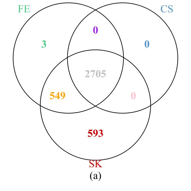
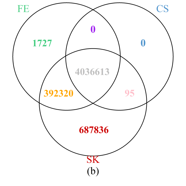
Figure 6 Venn diagrams of the numbers of DMCs detected by the three methods: (a) selected region of chromosome 1; (b) whole genome. Note that a site is declared to be a DMC if FDR ≤0.05.

5. Discussion

The FE test is still frequently used and recommended for analyzing BS-seq data to detect differentially methylated cytosines, an important topic in understanding biological and molecular mechanisms of diseases. In this study, we aimed to investigate whether an unconditional test for detecting DMCs is more appropriate than a conditional test, such as the FE test, due to the concern that the assumptions necessary for applying the FE test may be violated for BS-seq data. We were further intrigued by how spatial correlation and between-sample variability inherent in patient samples would affect the performance of the methods.

Our extensive simulation and theoretical analyses indicate that the unconditional SK test is indeed more powerful for detecting DMCs than the conditional FE test, echoing mounting evidence reported in general settings [44,45]. This conclusion has also been corroborated by the application of these tests to a BS-seq dataset. In particular, the SK test has a greater ability for detecting differential methylation with limited sequencing depth or smaller differences. It is interesting to note that in our real data analysis, we considered methylation in the context of CHG and CHH, in addition to CpG. Although not within the scope of the current study, it would be of considerable interest to the wider scientific community to investigate whether the SK test also outperforms the other two methods in investigating DNA methylation in plants, where it is known that methylation levels in the context of CHH are much lower than those in the context of CpG. We plan to undertake this task in a future study.

As expected, when variability exists between samples within a condition, the three methods explored inevitably suffer from inflated type I error. The power of these methods also decreases slightly as between-sample variability increases. The t-test, on the other hand, controls type I error well, although it generally has low power and the power loss with increasing variability is much more drastic compared to that of the other methods. Therefore, even though the t-test is appropriate for analyzing BS-seq data in the presence of between-sample variability, its low power precludes it from being a method of choice. Instead, if spatial correlation and between-sample variability do exist, it is likely that recently proposed methods based on advanced models rather than the classical ones reviewed here would be more appropriate [41,42,46,47,48]. In particular, when covariate information is available and needs to be incorporated to avoid confounding, then none of the methods discussed here are amenable to that situation. As such, recent state-of-the-art methods [2,48] are needed to deal with this issue appropriately.

Although not within the scope of the current study, which focuses on classical statistical methods, we nevertheless also considered a dataset analyzed in a model-based method (MOABS) [49] and compared the results from the three classical methods discussed here with those from MOABS as a further illustration. The data consist of two replicates of cases and two replicates of controls from a study of mouse methylomes and are contained in the MOABS package. As shown in Supplementary Figure S9, the results demonstrate that the SK test is more powerful than the FE and CS tests, which is consistent with all the other results presented here. On the other hand, an almost equal number of unique DMCs were identified by the SK test and MOABS, which once again demonstrates the relevance of the SK test even when more advanced methodologies are available, especially in situations where there is likely to be limited between-sample variability. Of course, a general conclusion is not warranted on the basis of a single analysis; therefore; further work is required to quantify the relative merits of these two sets of methods.

If site-by-site analysis of BS-seq data is desired when there is a single sample or when there is minimal between-sample variability, then the SK test is recommended as assumptions that are inconsistent with the data generation process are not necessary. Although it is indeed computationally more expensive compared to the FE and CS tests, the SK test it is still computationally feasible. Source code for the KS test. The Storer–Kim method was implemented in the WRS2 R-package, which is freely available on CRAN: https://cran.r-project.org/web/packages/WRS2/.

Acknowledgments

This work was supported in part by the National Science Foundation grant DMS-1208968 and NIGMS grant R01GM114142. The authors would like to thank the anonymous referees for their constructive comments.

Additional Materials

The following additional materials are uploaded at the page of this paper.

1. Figure S1: Heatmaps of P-values and rejection regions (those with P-values ≤0.05; shaded in black): (a) Storer–Kim (SK); (b) Fisher’s exact (FE); and (c) and chi-squared (CS) tests. The results are for a pair of p’s fixed at p₁ = 0.6 and p₂ = 0.4. For each method, the rejection region is the combination of (n₁,n₂) (in the range of 1-100) for which the DMC is declared. Note that the jagged line in (b) is due to the discrete nature of the FE test.

2. Figure S2: Heatmaps of P-values and rejection regions (those with P-values ≤0.05; shaded in black): (a) Storer–Kim (SK); (b) Fisher’s exact (FE); and (c) and chi-squared (CS) tests. The results are for a pair of p’s fixed at p₁ = 0.75 and p₂ = 0.25. For each method, the rejection region is the combination of (n₁,n₂) (in the range of 1-100) for which the DMC is declared. Note that the jagged line in (b) is due to the discrete nature of the FE test.

3. Figure S3: Heatmaps of P-values and rejection regions (those with P-values ≤0.05; shaded in black): (a) Storer–Kim (SK); (b) Fisher’s exact (FE); and (c) and chi-squared (CS) tests. The results are for a pair of p’s fixed at p₁ = 0.8 and p₂ = 0.6. For each method, the rejection region is the combinations of (n₁,n₂) (in the range of 1-100) for which DMC is declared. Note that the jagged line in (b) is due to the discrete nature of the FE test.

4. Figure S4: Heatmaps of P-values and rejection regions (those with P-values ≤0.05; shaded in black): (a) Storer–Kim (SK); (b) Fisher’s exact (FE); and (c) and chi-squared (CS) tests. The results are for a scenario in which the total number of reads is 50 in both samples. For each method, the rejection region is the combination of (p₁,p₂) (in the range of 0-1) for which the DMC is declared. Note that the jagged line in (b) is due to the discrete nature of the FE test.

5. Figure S5: Heatmaps of P-values and rejection regions (those with P-values ≤0.05; shaded in black): (a) Storer–Kim (SK); (b) Fisher’s exact (FE); and (c) and chi-squared (CS) tests. The results are for a scenario in which the total numbers of reads are 40 and 10 in the two samples. For each method, the rejection region is the combination of (p₁,p₂) (in the range of 0-1) for which the DMC is declared. Note that the jagged line in (b) is due to the discrete nature of the FE test.

6. Figure S6: Heatmaps of P-values and rejection regions (those with P-values ≤0.05; shaded in black): (a) Storer–Kim (SK); (b) Fisher’s exact (FE); and (c) and chi-squared (CS) tests. The results are for a scenario in which the total numbers of reads are 80 and 20 in the two samples. For each method, the rejection region is the combination of (p₁,p₂) (in the range of 0-1) for which the DMC is declared. Note that the jagged line in (b) is due to the discrete nature of the FE test.

7. Figure S7: Venn diagrams of numbers of DMCs detected by three methods chromosome-by-chromosome. Note that a site is designated a DMC if the chromosome-wise FDR ≤0.05.

8. Figure S8: Histogram of the read counts for chromosomes 1–22, X, and Y from the H1 (top) and I90 (bottom) cell lines.

9. Figure S9: Venn diagram of the numbers of DMCs detected by three classical methods, FE, CS, SK, and a newer method, MOABS. For the classical methods, a site is designated a DMC if FDR ≤0.05. For MOABS, a site is designated a DMC if its credible methylation difference (CDIF) is greater than 0.2, a threshold suggested in the software.

Author Contributions

SL conceived the idea of the project and designed the studies. HL carried out all the analyses. SL and HL wrote the manuscript.

Competing Interests

The authors have declared that no competing interests exist.

References

- Lister R, Pelizzola M, Dowen RH, Hawkins RD, Hon G, Tonti-Filippini J, et al. Human DNA methylomes at base resolution show widespread epigenomic differences. Nature. 2009; 462: 315. [CrossRef] [Google scholar] [PubMed]
- Hebestreit K, Dugas M, Klein H-U. Detection of significantly differentially methylated regions in targeted bisulfite sequencing data. Bioinformatics. 2013; 29: 1647-1653. [CrossRef] [Google scholar] [PubMed]
- Eckhardt F, Lewin J, Cortese R, Rakyan VK, Attwood J, Burger M, et al. DNA methylation profiling of human chromosomes 6, 20 and 22. Nature Genet. 2006; 38: 1378. [CrossRef] [Google scholar] [PubMed]
- Suzuki MM, Bird A. DNA methylation landscapes: provocative insights from epigenomics. Nat Rev Genet. 2008; 9: 465. [CrossRef] [Google scholar] [PubMed]
- Deaton AM, Bird A. CpG islands and the regulation of transcription. Genes Dev. 2011; 25: 1010-1022. [CrossRef] [Google scholar] [PubMed]
- Hansen KD, Timp W, Bravo HC, Sabunciyan S, Langmead B, McDonald OG, et al. Increased methylation variation in epigenetic domains across cancer types. Nature Genet. 2011; 43: 768. [CrossRef] [Google scholar] [PubMed]
- Vogelstein B, Papadopoulos N, Velculescu VE, Zhou S, Diaz LA, Kinzler KW. Cancer genome landscapes. science. 2013; 339: 1546-1558. [CrossRef] [Google scholar] [PubMed]
- Das PM, Singal R. Biology of neoplasia. J Clin Oncol. 2004; 22: 4632-4642. [CrossRef] [Google scholar] [PubMed]
- Fearon ER. Molecular genetics of colorectal cancer. Annu Rev Pathol. 2011; 6: 479-507. [CrossRef] [Google scholar] [PubMed]
- Bonder MJ, Luijk R, Zhernakova DV, Moed M, Deelen P, Vermaat M, et al. Disease variants alter transcription factor levels and methylation of their binding sites. Nature Genet. 2017; 49: 131. [CrossRef] [Google scholar] [PubMed]
- Chatterjee A, Stockwell PA, Rodger EJ, Morison IM. Comparison of alignment software for genome-wide bisulphite sequence data. Nucleic Acids Res. 2012; 40: e79. [CrossRef] [Google scholar] [PubMed]
- Xi Y, Li W. BSMAP: whole genome bisulfite sequence MAPping program. BMC Bioinformatics. 2009; 10: 232. [CrossRef] [Google scholar] [PubMed]
- Wu TD, Nacu S. Fast and SNP-tolerant detection of complex variants and splicing in short reads. Bioinformatics. 2010; 26: 873-881. [CrossRef] [Google scholar] [PubMed]
- Krueger F, Andrews SR. Bismark: a flexible aligner and methylation caller for Bisulfite-Seq applications. Bioinformatics. 2011; 27: 1571-1572. [CrossRef] [Google scholar] [PubMed]
- Harris EY, Ponts N, Levchuk A, Roch KL, Lonardi S. BRAT: bisulfite-treated reads analysis tool. Bioinformatics. 2009; 26: 572-573. [CrossRef] [Google scholar] [PubMed]
- Liao W-W, Yen M-R, Ju E, Hsu F-M, Lam L, Chen P-Y. MethGo: a comprehensive tool for analyzing whole-genome bisulfite sequencing data. BMC Genomics. 2015; 16: S11. [CrossRef] [Google scholar] [PubMed]
- Huang X, Zhang S, Li K, Thimmapuram J, Xie S. ViewBS: a powerful toolkit for visualization of high-throughput bisulfite sequencing data. Bioinformatics. 2017; 34: 708-709. [CrossRef] [Google scholar] [PubMed]
- Shafi A, Mitrea C, Nguyen T, Draghici S. A survey of the approaches for identifying differential methylation using bisulfite sequencing data. Brief Bioinform. 2017. [Google scholar]
- Han C, Tang H, Lou S, Gao Y, Cho MH, Lin S. Evaluation of recent statistical methods for detecting differential methylation using BS-seq data. 2018; 2: DOI: 10.21926/obm.genet.1804041 [CrossRef] [Google scholar]
- Teschendorff AE, Relton CL. Statistical and integrative system-level analysis of DNA methylation data. Nat Rev Genet. 2018; 19: 129. [CrossRef] [Google scholar] [PubMed]
- Bock C. Analysing and interpreting DNA methylation data. Nat Rev Genet. 2012; 13: 705. [CrossRef] [Google scholar] [PubMed]
- Ayyala DN, Frankhouser DE, Ganbat J-O, Marcucci G, Bundschuh R, Yan P, et al. Statistical methods for detecting differentially methylated regions based on MethylCap-seq data. Brief Bioinform. 2015; 17: 926-937. [CrossRef] [Google scholar] [PubMed]
- Jaffe AE, Feinberg AP, Irizarry RA, Leek JT. Significance analysis and statistical dissection of variably methylated regions. Biostatistics. 2011; 13: 166-178. [CrossRef] [Google scholar] [PubMed]
- McCarthy DJ, Chen Y, Smyth GK. Differential expression analysis of multifactor RNA-Seq experiments with respect to biological variation. Nucleic Acids Res. 2012; 40: 4288-4297. [CrossRef] [Google scholar] [PubMed]
- Qin Z, Li B, Conneely KN, Wu H, Hu M, Ayyala D, et al. Statistical challenges in analyzing methylation and long-range chromosomal interaction data. Stat Biosci. 2016; 8: 284-309. [CrossRef] [Google scholar] [PubMed]
- Wagner JR, Busche S, Ge B, Kwan T, Pastinen T, Blanchette M. The relationship between DNA methylation, genetic and expression inter-individual variation in untransformed human fibroblasts. Genome Biol. 2014; 15: R37. [CrossRef] [Google scholar] [PubMed]
- Wen Y, Chen F, Zhang Q, Zhuang Y, Li Z. Detection of differentially methylated regions in whole genome bisulfite sequencing data using local Getis-Ord statistics. Bioinformatics. 2016; 32: 3396-3404. [CrossRef] [Google scholar] [PubMed]
- Mehrotra DV, Chan IS, Berger RL. A cautionary note on exact unconditional inference for a difference between two independent binomial proportions. Biometrics. 2003; 59: 441-450. [CrossRef] [Google scholar] [PubMed]
- Greenland S. On the logical justification of conditional tests for two-by-two contingency tables. Am Stat. 1991; 45: 248-251. [Google scholar]
- Andrés AM, Mato AS. Choosing the optimal unconditioned test for comparing two independent proportions. Comput Stat Data Anal. 1994; 17: 555-574. [CrossRef] [Google scholar]
- D‘agostino RB, Chase W, Belanger A. The appropriateness of some common procedures for testing the equality of two independent binomial populations. Am Stat. 1988; 42: 198-202. [Google scholar]
- Upton GJ. A comparison of alternative tests for the 2× 2 comparative trial. J R Stat Soc Series A. 1982: 86-105. [CrossRef] [Google scholar]
- Little RJ. Testing the equality of two independent binomial proportions. Am Stat. 1989; 43: 283-288. [Google scholar]
- Hope AC. A simplified Monte Carlo significance test procedure. J R Stat Soc Series B. 1968: 582-598. [CrossRef] [Google scholar]
- Storer BE, Kim C. Exact properties of some exact test statistics for comparing two binomial proportions. J Am Stat Assoc. 1990; 85: 146-155. [CrossRef] [Google scholar]
- Suissa S, Shuster JJ. The 2 x 2 matched-pairs trial: exact unconditional design and analysis. Biometrics. 1991: 361-372. [CrossRef] [Google scholar]
- Barnard G. A new test for 2× 2 tables. Nature. 1945; 156: 177. [CrossRef] [Google scholar]
- Yates F. Contingency tables involving small numbers and the χ 2 test. J Royal Stat Soc. 1934; 1: 217-235. [CrossRef] [Google scholar]
- Lydersen S, Fagerland MW, Laake P. Recommended tests for association in 2× 2 tables. Stat Med. 2009; 28: 1159-1175. [CrossRef] [Google scholar] [PubMed]
- Satterthwaite FE. An approximate distribution of estimates of variance components. Biometrics. 1946; 2: 110-114. [CrossRef] [Google scholar]
- Park J, Lin S. Detection of Differentially Methylated Regions Using Bayesian Curve Credible Bands. Stat Biosci. 2018; 10: 20-40. [CrossRef] [Google scholar]
- Hansen KD, Langmead B, Irizarry RA. BSmooth: from whole genome bisulfite sequencing reads to differentially methylated regions. Genome Biol. 2012; 13: R83. [CrossRef] [Google scholar] [PubMed]
- NIH, “NFASC gene entry from NIH network. Available from: https://www.ncbi.nlm.nih.gov/gene/23114.
- Berger R. Power comparison of exact unconditional tests for comparing two binomial proportions. Institute of Statistics Mimeo Series. 1994. [Google scholar]
- Krishnamoorthy K, Thomson J. Hypothesis testing about proportions in two finite populations. Am Stat. 2002; 56: 215-222. [CrossRef] [Google scholar]
- Feng H, Conneely KN, Wu H. A Bayesian hierarchical model to detect differentially methylated loci from single nucleotide resolution sequencing data. Nucleic Acids Res. 2014; 42: e69-e69. [CrossRef] [Google scholar] [PubMed]
- Park Y, Figueroa ME, Rozek LS, Sartor MA. MethylSig: a whole genome DNA methylation analysis pipeline. Bioinformatics. 2014; 30: 2414-2422. [CrossRef] [Google scholar] [PubMed]
- Dolzhenko E, Smith AD. Using beta-binomial regression for high-precision differential methylation analysis in multifactor whole-genome bisulfite sequencing experiments. BMC Bioinformatics. 2014; 15: 215. [CrossRef] [Google scholar] [PubMed]
- Sun D, Xi Y, Rodriguez B, Park HJ, Tong P, Meong M, et al. MOABS: model based analysis of bisulfite sequencing data. Genome Biol. 2014; 15: R38. [CrossRef] [Google scholar] [PubMed]